Handling Spike Traffic Reliably: Improvement
This post is an extension of “Handling Spike Traffic Reliably: Implementation”, covering the problems we encountered during production operation and the improvements we made.
Channel.io is a B2B product used by approximately 200,000 customers, and many of its key features involve large-scale spike loads (internally called bulk actions). Consider the following scenarios:
- Uploading ~1 million customer records to Channel.io
- Running a promotion targeting 100,000 customers whose recent purchase amount exceeds $10
- Bulk-applying an ‘A’ tag to all conversations from the past year
Overview
Channel.io is a B2B SaaS product serving approximately 220,000 customers, and it must reliably process anywhere from hundreds to millions of items per request. The bulk action server processes requests within a defined TPS through rate limit throttling and HOL blocking minimization.
However, when there are many long-lived jobs, all workers can become busy, causing HOL blocking to resurface. During initial operations, developers manually adjusted worker counts, but since this was dependent on client request patterns, automatic scaling was necessary.
1. Dynamic Scaling
The Problem
Even with a fair queue in place, if the worker count itself is insufficient, the job queue depth grows. Jobs in the bulk action server are essentially bundles of multiple operations, so execution times can extend to several seconds. This causes busy workers to pile up, and while TPS is maintained, jobs aren’t being placed into the non-ready queue — leading to many delayed jobs and tail latency.
Finding the Right Metric
We experimented with several scaling trigger candidates:
1. Ready Queue Size (number of waiting tasks)
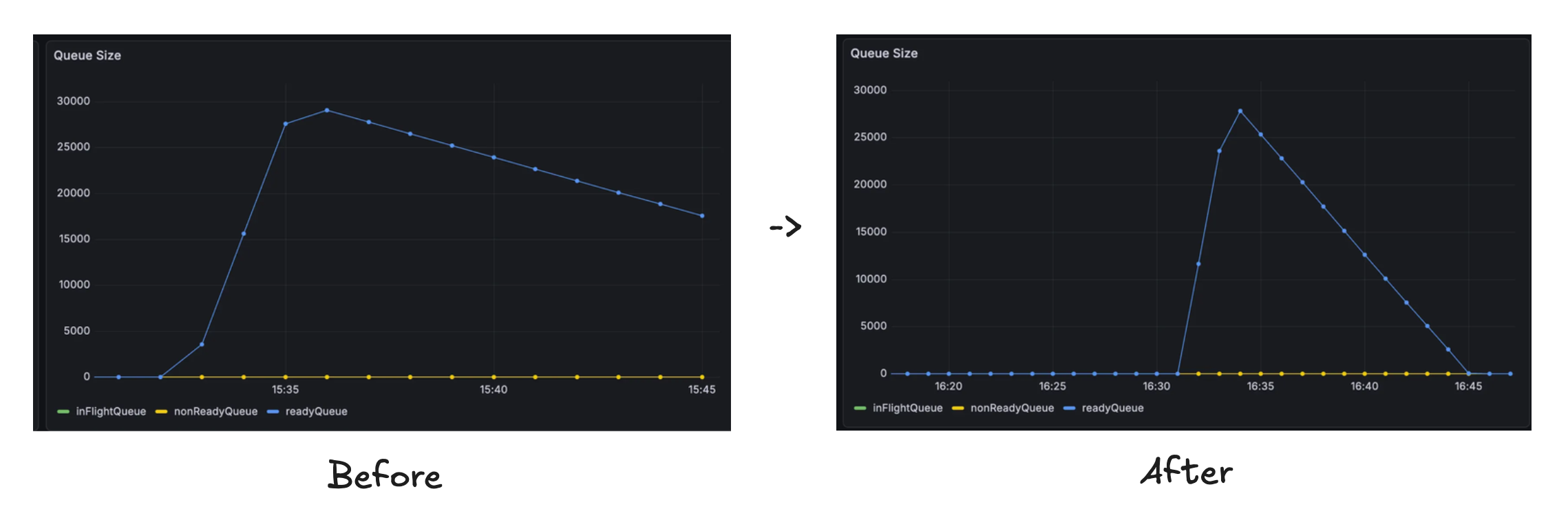
The most intuitive metric. Processing 100,000 items with 8 workers took 25 minutes, and doubling workers when queue size exceeded 10,000 reduced this to 14 minutes.
However, during the initial rate limit exploration phase, queue size spikes regardless of actual load. Scaling up workers at this point only adds workers that hit the rate limit and do nothing.
2. In-Flight Queue Size (number of executing tasks)
Tasks throttled by rate limiting also pass through the in-flight state, so this metric doesn’t accurately reflect actual worker load. It simply increased linearly with worker count.
3. Job Execution Latency (p95)
This can only be measured from already-executing tasks, making it difficult to use as a leading indicator. You can’t know a waiting task’s execution time until you actually process it.
Key Metric
Per-Worker Queue Depth = ratio = queueDepth / currentWorkers
Among the candidates, we chose Per-Worker Queue Depth (PWQD). The same queue size means different things depending on the number of workers. A queue of 100 items with 8 workers means 12.5 per worker — high load. With 64 workers, it’s 1.6 per worker — comfortable.
When this ratio consecutively exceeds a threshold, it triggers scale-up. The “consecutively” condition prevents overreaction to momentary spikes.
Scaling Algorithm
Characteristics of bulk action jobs:
- Long-lived jobs are possible
- Spiky request patterns
- Long total execution time while maintaining TPS
Since PWQD spikes at the time of bulk action registration, the algorithm must be sensitive to spiky traffic but conservative during the initial registration phase.
Experiment 0: Ratio-Based Exponential Scaling
When the PWQD metric exceeds the threshold, worker count increases exponentially. This responds well to high traffic, but exhibited large oscillation during scale-down. Rejected.
Experiment 1: Congestion Control-Based Algorithm
Inspired by TCP AIMD — doubling during the Slow Start phase and increasing linearly after ssthresh. Oscillation was reduced, but while it responded immediately to initial requests, it was overly conservative for subsequent requests.
Experiment 2: Exponential & Time Decay
Scale up when PWQD remains persistently high, and apply time decay for conservative scale-down. The slow decrease prepares for additional requests, enables fast worker increases, and avoids oscillation. It responds quickly enough to additional requests.
Dynamic Scaling — Results
Through these improvements, we could handle actual traffic within appropriate TPS compliance. We reduced the scope of developer attention — now they only need to decide whether to scale up machines or increase the maximum worker count based on key metrics.
However, partitioning was additionally required. Why did we need to sacrifice complexity to apply partitioning?
2. Horizontal Scaling: Partitioning
Partitioning is an option considered for horizontal scaling when the workload exceeds what a single machine can handle. While instance scaling partially solved the issue, we needed a structure that enables easy horizontal scaling through partitioning in the long term.
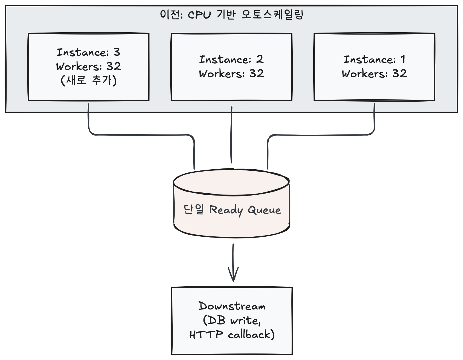
Partitioning also adds predictability to dynamic scaling. The previous approach scaled by adding instances with fixed worker counts based on CPU utilization. Even when only 10 workers were needed, adding one instance (32 workers) meant worker counts jumped in multiples: 32 → 64 → 96. By fixing the number of consumers per partition and relying solely on worker count scaling, we simplified the complexity.
Between Complexity and Scalability
Partitioning requires implementing distributed coordination mechanisms like membership management and leader election. However, the current job queue TPS isn’t that high.
The bulk action server shares Redis with Channel.io’s main service, and Redis CPU utilization had plenty of headroom. The main concern was scaling workers and bulk action instances.
Therefore, we proceeded with partitioning the job queue consumers. The goal was to establish a partition-aware structure in preparation for future Redis traffic growth, and to create a scalable structure by deploying consumers through logical partitioning.
Implementation Details
Partitioning Criteria
When applying partitioning, we needed to decide how to divide the work. There were three candidates:
1. Channel (Customer) Unit
All bulk actions for the same customer are placed in the same partition. This makes it easy to trace failures and allows natural priority comparison between tasks within the same customer. However, if a large customer’s multiple bulk actions concentrate on one partition, that partition becomes overloaded, affecting other customers in the same partition as well.
2. Bulk Action Type Unit
Dividing by operation type — “send message,” “close conversation,” etc. Useful when a specific type generates heavy load, but since scale varies enormously within the same type (10 items vs. 1 million items), the isolation effect is limited.
A multi-level strategy isolating top-traffic types is viable, but to reduce management complexity, we explored a structure that doesn’t depend on user request patterns. Since types are defined by the client, using them as partitioning criteria would make the bulk action server dependent on client type definitions.
3. TaskGroup (Bulk Action) Unit
Each bulk action request is independently distributed across partitions. The fine-grained distribution unit leads to more even load distribution across partitions. Even if a large customer submits multiple bulk actions simultaneously, each request can be distributed to different partitions, mitigating the phenomenon of load concentrating on specific partitions.
We chose TaskGroup unit partitioning. While channel-unit partitioning is generally preferred, if a customer heavily uses bulk actions, they’d be penalized simply for being in the same partition. A structure where requests always go to the same partition won’t work. We applied TaskGroup-level partitioning to properly distribute load.
In Channel.io’s bulk action system, what we want to isolate isn’t “a specific customer” but “a specific large-scale request” itself. If a single bulk action of 1 million items is the problem, isolating that bulk action is the most direct solution. Other bulk actions may end up in the same partition, but if partitions are sufficiently divided, the scope of impact from large requests is limited from the entire system to just a few partitions.
Logical Partitioning
As we determined earlier, Redis machine performance itself was sufficient. The bulk action server shares Redis with Channel.io’s main service, and checking actual Redis CPU utilization confirmed there was headroom.
So where was the problem? Not in Redis get/set performance, but in the structure itself where multiple TaskGroups share a single Ready Queue.
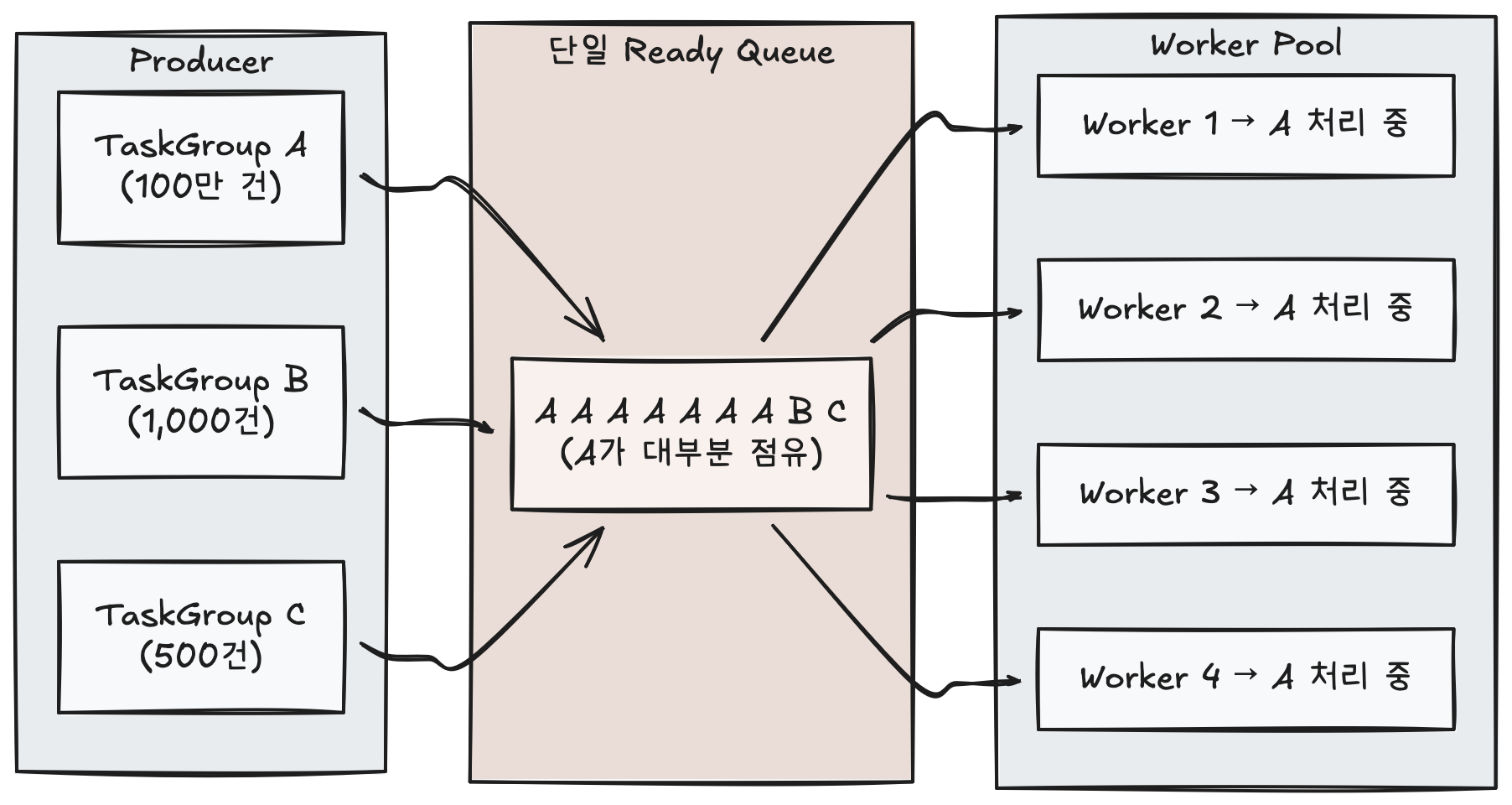
Without partitioning, all TaskGroup tasks are loaded into a single Ready Queue (Redis Sorted Set). When a large TaskGroup’s (e.g., 1 million items) tasks pile up in the queue, workers focus on processing those tasks, delaying other TaskGroups’ tasks. Priority-based sorting exists, but it can’t overcome sheer volume differences.
Since Redis performance is sufficient, the solution is separating keyspaces within the same Redis — that is, splitting into multiple queues.
Before: /{stage}/queue/{resourceKey}                ← single queue
After:  /{stage}/queue/partition_{id}/{resourceKey} ← independent queues per partition
Rather than physically separating Redis instances (Redis Cluster), we create independent queues by separating only the key prefix within the same Redis. This is why we call it “logical partitioning.”
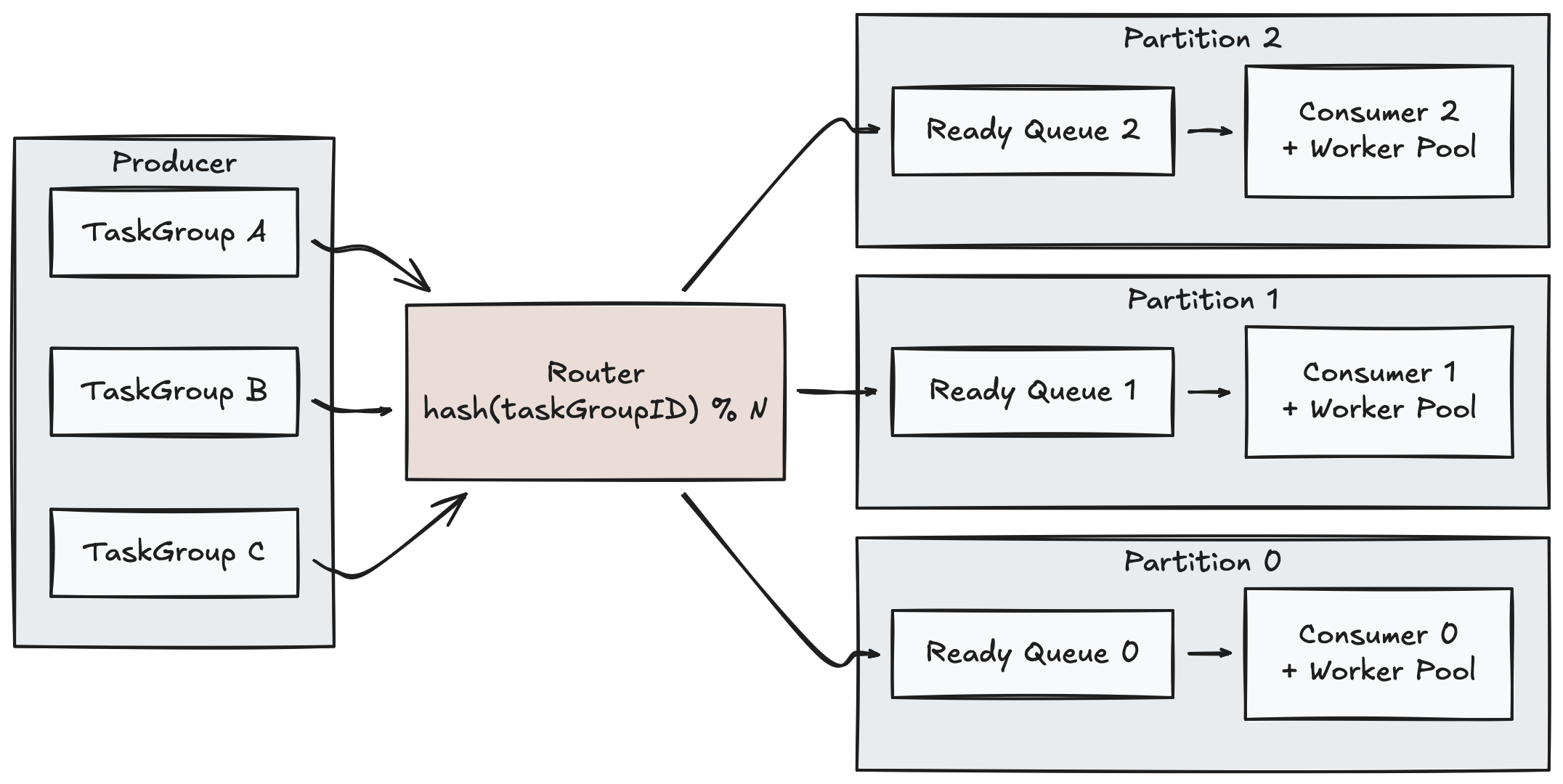
The key to routing is using taskGroupID as the partition key. Tasks from the same TaskGroup are always routed to the same partition via hash(taskGroupID) % N, and each partition has an independent Consumer + Worker pipeline. Since a TaskGroup never spreads across multiple partitions, priority management and state tracking at the TaskGroup level within a partition happens naturally. Even if TaskGroup A’s massive tasks pile up in Partition 0, processing in Partitions 1 and 2 is unaffected.
We introduced an abstraction layer called the Queue Pool to minimize changes to existing business logic. Producers only need to add one partition key parameter to the existing queue.Enqueue(item) call, and consumers receive their partition’s queue at initialization time and operate identically to before — no changes needed. All complexity related to routing and partition selection is encapsulated within the Queue Pool.
Simplifying Scaling Complexity
Let’s compare how partitioning solves the instance-level scaling problem described earlier.
After introducing partitioning, we fix one consumer per partition and dynamically adjust only the worker (goroutine) count within each process.
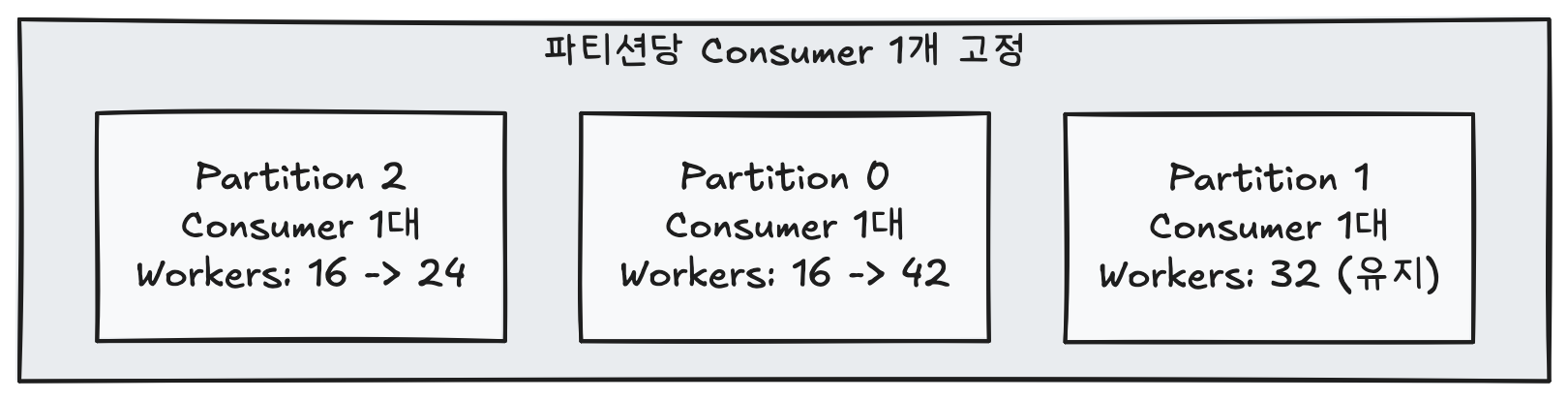
Since the worker count adjustment API was already implemented, we can increase or decrease workers as needed. Instance count doesn’t change, and each partition scales independently without interfering with others.
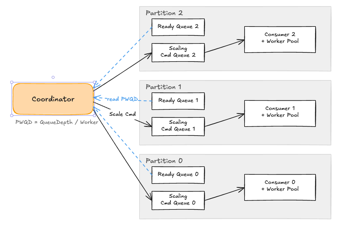
So who decides each partition’s worker count? The Coordinator handles this role. The Coordinator periodically traverses all partitions, independently observes each partition’s load state, and when it determines scaling is needed, issues a command to that partition’s Scaling Command Queue. Consumers watch their Command Queue and adjust worker counts when commands arrive.
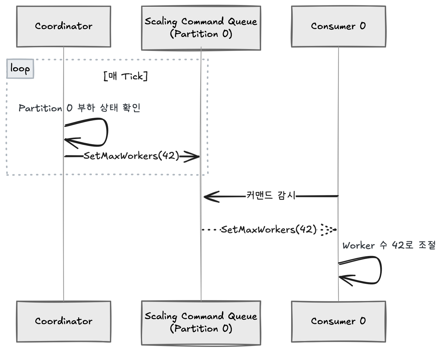
The Coordinator only observes and decides — actual execution is performed independently by each Consumer. Thanks to this structure, scaling occurs without inter-partition interference.
One more consideration: when a Consumer process restarts while dynamic scaling has adjusted worker counts, it has no way of knowing how many workers it was previously using. Starting with default values means unnecessary time until scaling converges again. To solve this, we periodically save (checkpoint) each partition’s worker count to Redis and restore it on restart. Since checkpoint keys are separated by partition, only the relevant partition’s checkpoint needs to be read when a specific Consumer restarts.
Extending to Physical Partitioning
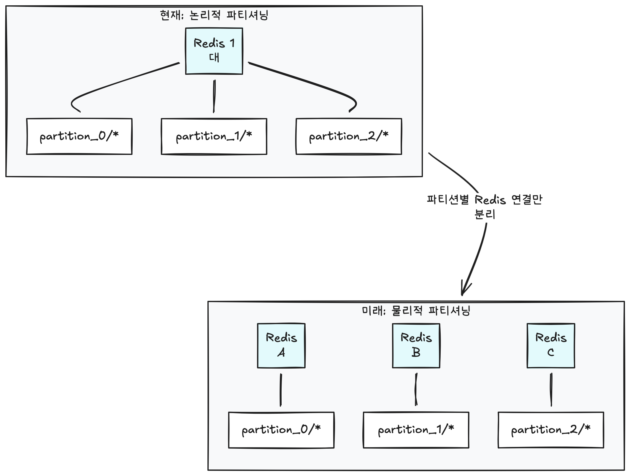
Logical partitioning is sufficient for now, but if Redis itself becomes overloaded in the future, physical partitioning (separating Redis instances) may be necessary. The current structure makes this transition straightforward.
Why the transition is straightforward:
- Keyspaces are already fully separated as
/queue/partition_{id}/, with no cross-key dependencies between partitions. - The Queue Pool manages each partition’s queue independently, so physical separation can be achieved by simply changing the Redis connection target for each queue.
- Each Consumer already processes only one partition, so only the Redis connection address needs to be swapped.
In other words, the change scope is limited to Redis connection configuration in one place, and business logic operates without modification.
Deployment Strategy
With code ready, the remaining question was how to apply it to a running system. Enabling partitioning changes the Redis keyspace, so the core challenge was how to handle tasks remaining in the existing queue.
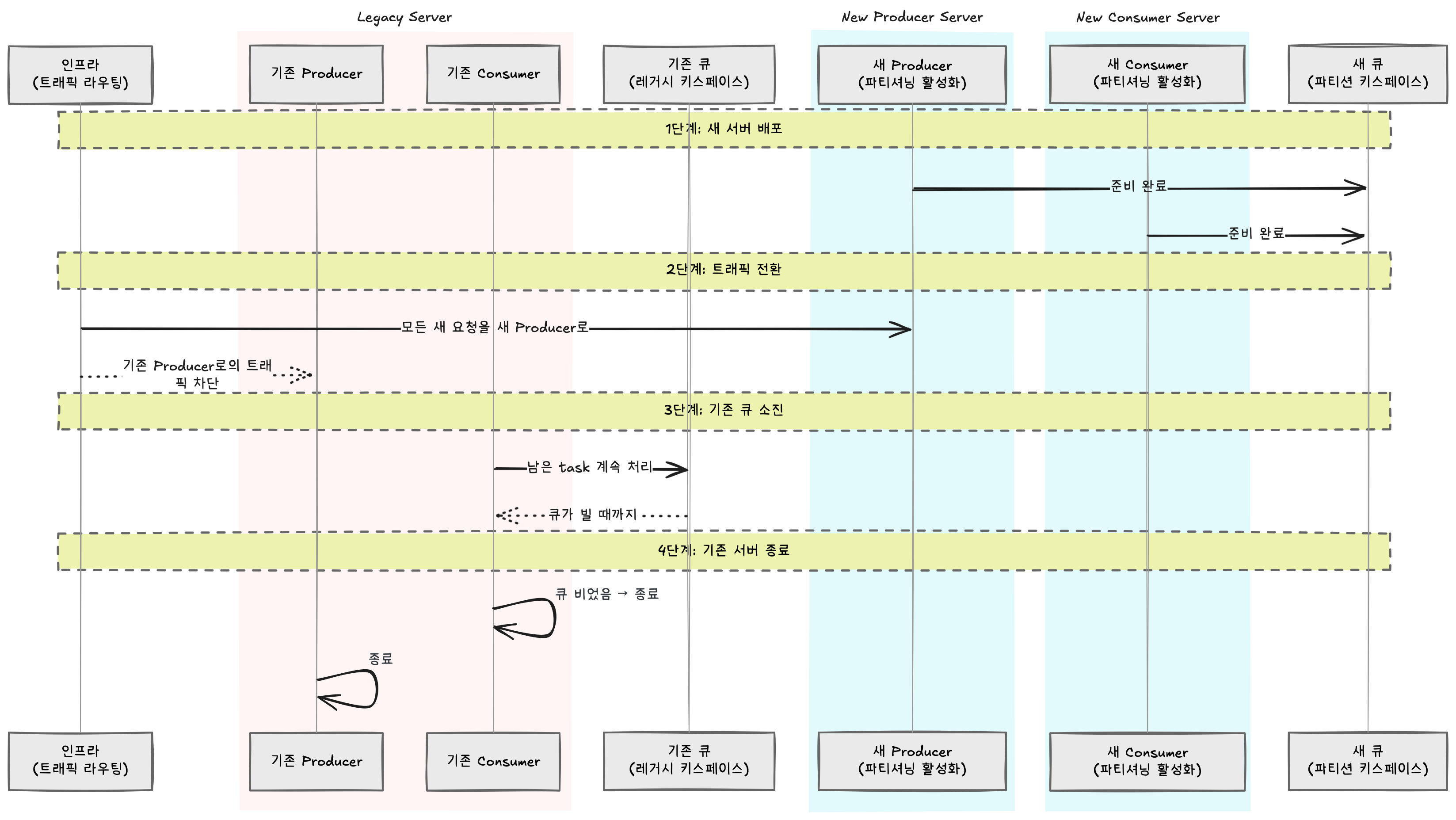
No separate data migration or drain-specific Consumer deployment was needed. By adjusting traffic routing at the infrastructure level, new requests were sent only to the new Producer, while existing servers naturally drained tasks from the legacy keyspace before shutting down. This was possible because backward compatibility was secured through a partitioning activation flag at the design stage. Servers with partitioning disabled and servers with it enabled can operate simultaneously since they use different key paths, avoiding conflicts.
Coordinator
The final component to introduce is the Coordinator. A coordinator is generally introduced to orchestrate partitioned or distributed systems, and it’s also a component that significantly increases complexity. However, introducing a coordinator was also a strategy for future extensibility.
We configured the coordinator to handle both scaling directives and state storage for consumers, with an eye toward the coordinator node taking on physical partitioning and partition expansion in the future. Still, this sacrifices system simplicity, so keeping the coordinator implementation as simple as possible was essential.
Therefore, the coordinator node implementation reuses the job queue infrastructure. This was heavily inspired by Kafka’s KRaft architecture.
Kafka and ZooKeeper
Kafka long delegated cluster metadata management (broker lists, partition leader election, configuration changes, etc.) to the external system ZooKeeper. This worked, but it meant operating two distributed systems — Kafka and ZooKeeper — increasing deployment, monitoring, and incident response complexity.
This problem was solved with the idea of “reusing the tools you already have.” Since what Kafka does best is writing and reading records to topics, metadata is also recorded as events in an internal topic (__cluster_metadata), and Controller nodes replicate this via Raft consensus. From a broker’s perspective, simply following the metadata topic — just as it normally consumes data topics — gives it the latest cluster state.
Instead of introducing a separate RPC channel or external coordination system (etcd, ZooKeeper, etc.) for the coordinator to communicate directives to consumers, we reused the existing job queue pipeline. The coordinator publishes scaling directive jobs to each partition’s job queue, and consumers poll in the same way as before — when they receive a command, they adjust worker counts or save their state.
As a result, the coordinator node tracks consumer states, collects PWQD metrics, and issues scaling directives. In practice, by reusing existing code, we were able to easily build the coordinator node with under 1,000 lines of code.
{
  "type": "SCALE_UP",
  "partition": 2,
  "targetWorkers": 24,
  "reason": "PWQD threshold exceeded for 3 consecutive cycles"
}
Results
Having covered the design and implementation of logical partitioning and dynamic scaling, we verified the improvements through a load test of 100,000 items.
Processing Performance
| Metric | Before | After |
|---|---|---|
| Processing time (100K items) | 25 minutes | 4 minutes |
| Improvement | — | 84% reduction |
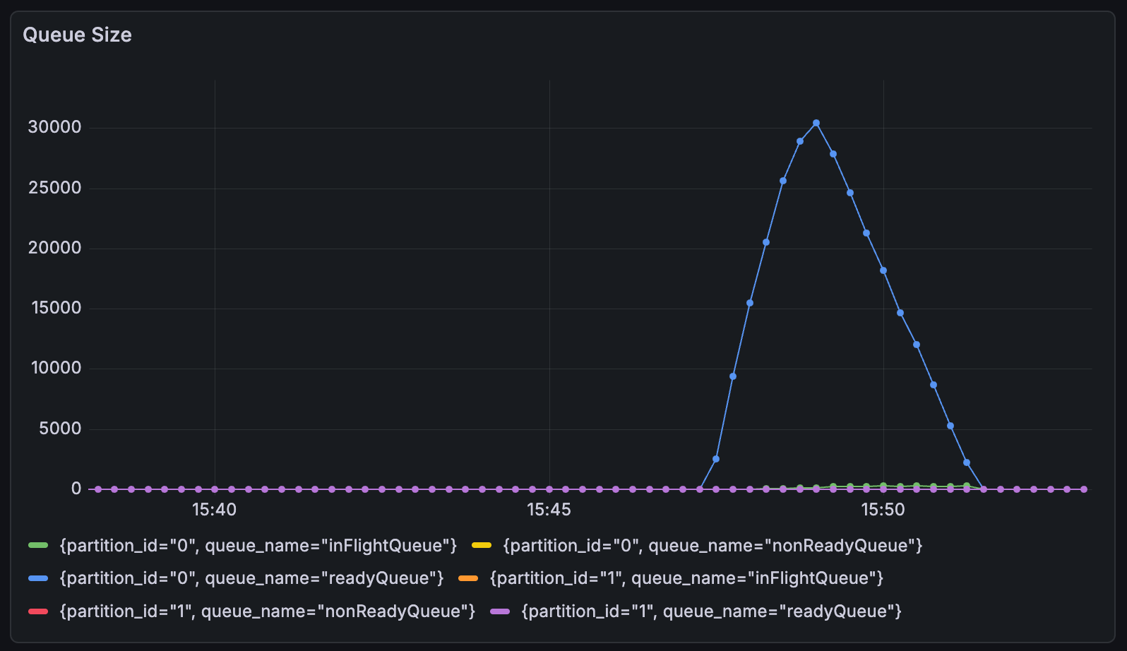
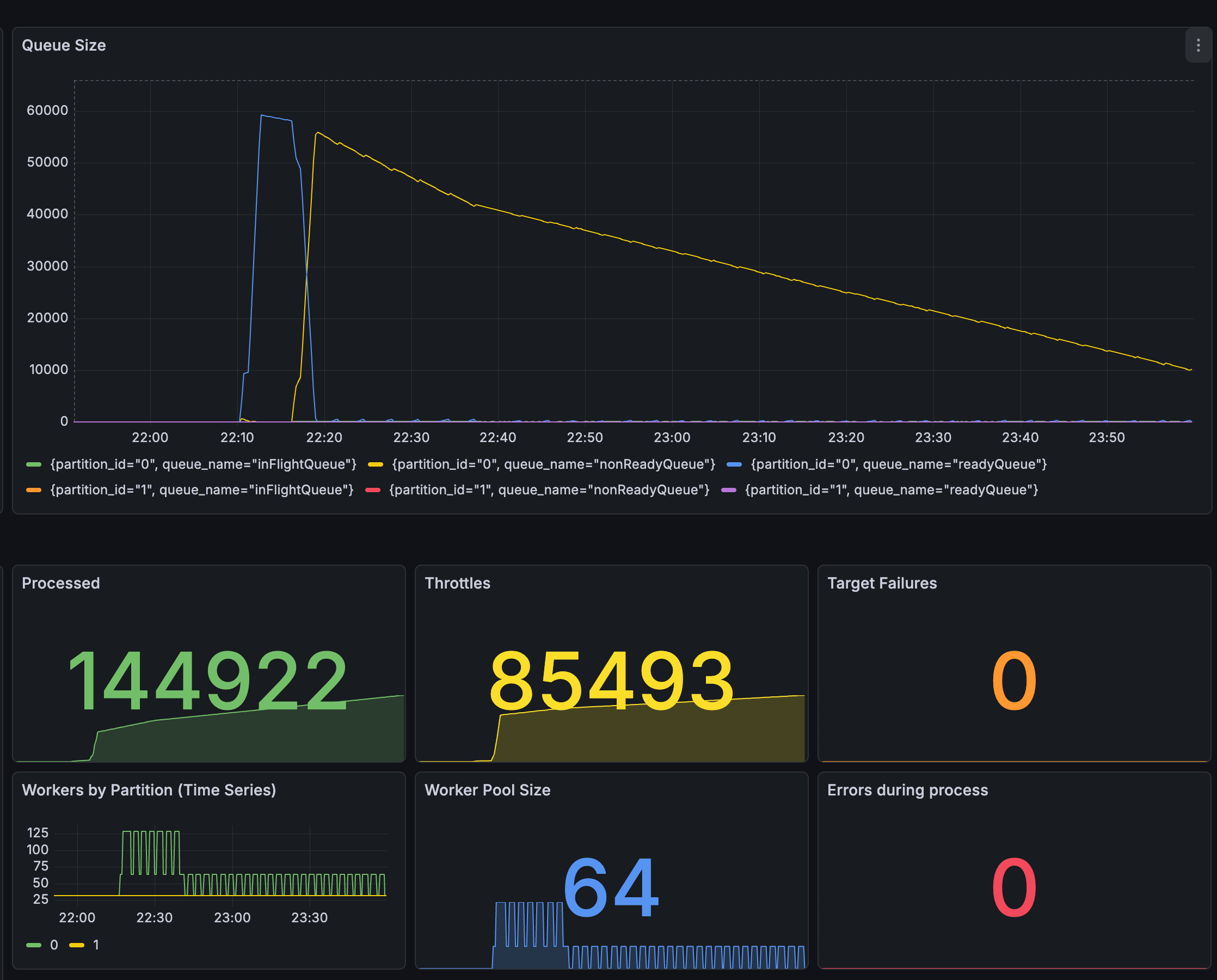
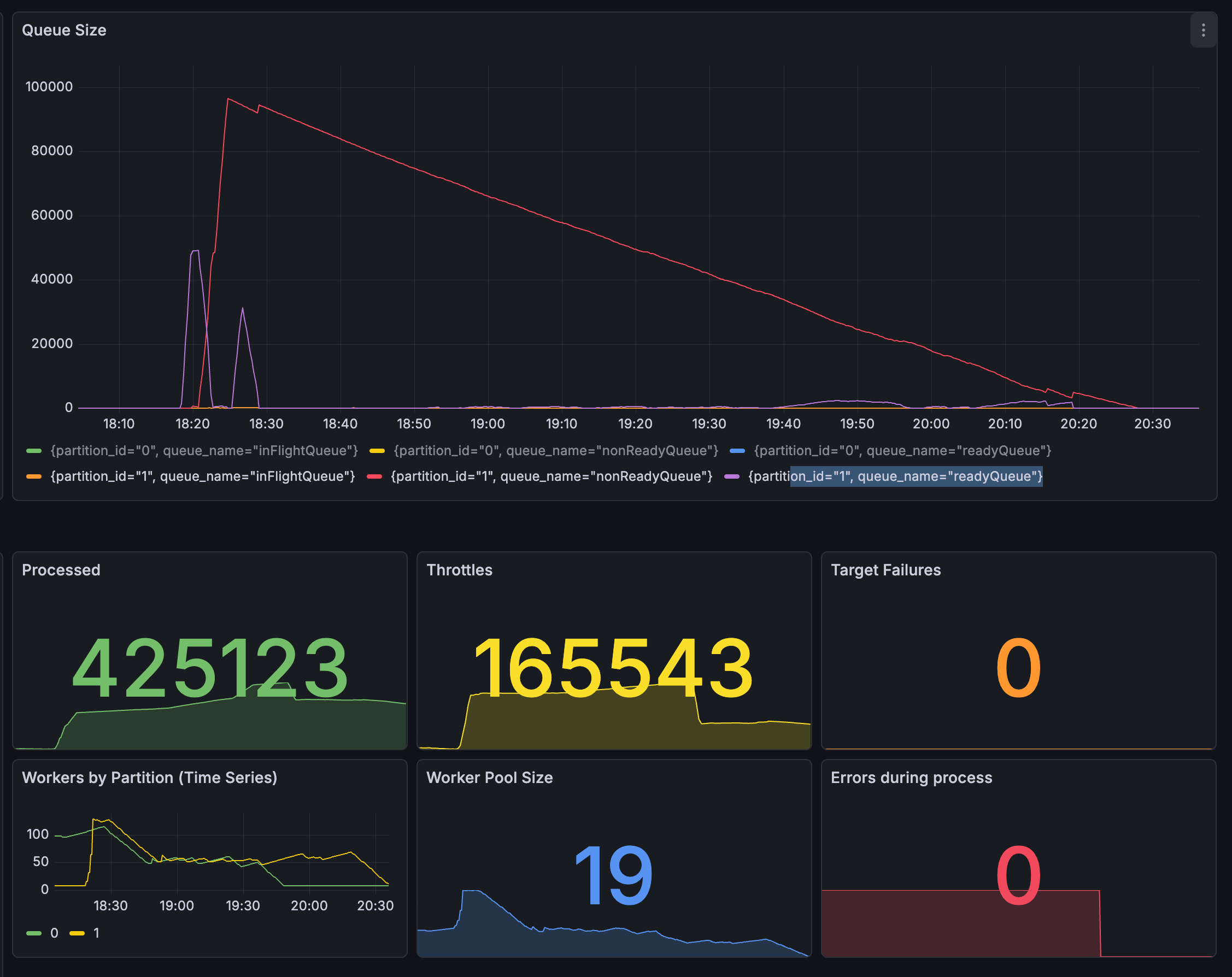
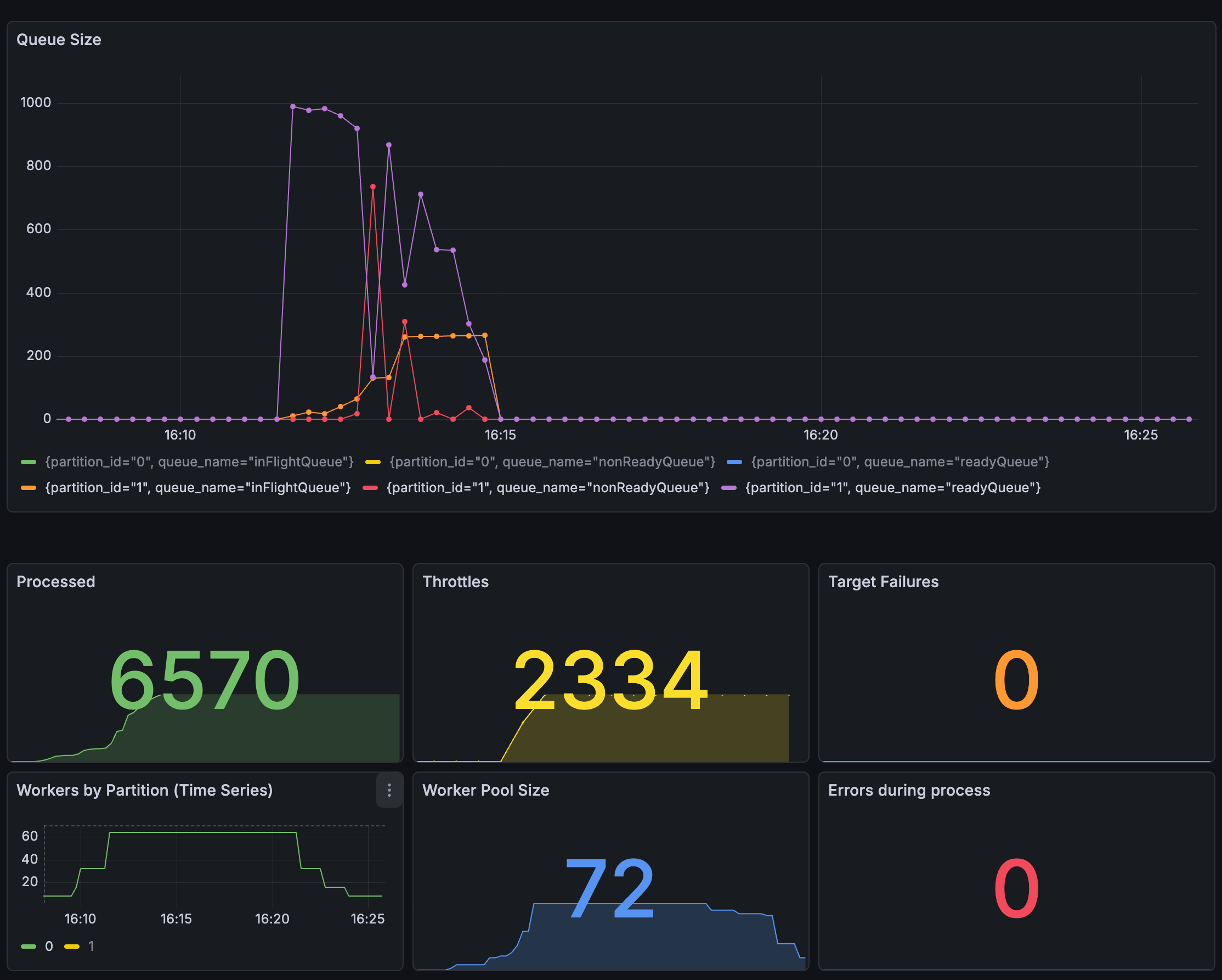
Partition Isolation Effect
We confirmed the resolution of HOL blocking — the core objective of partitioning. Previously, when a large TaskGroup occupied the queue, other TaskGroups’ processing was delayed. After partitioning, each partition operates independently, so even if a specific partition is flooded with large tasks, processing in other partitions is unaffected.
Dynamic Scaling
Unlike the previous instance-level jumps (32 → 64 → 96), we confirmed that the Coordinator’s dynamic scaling increases or decreases workers per partition only as needed.
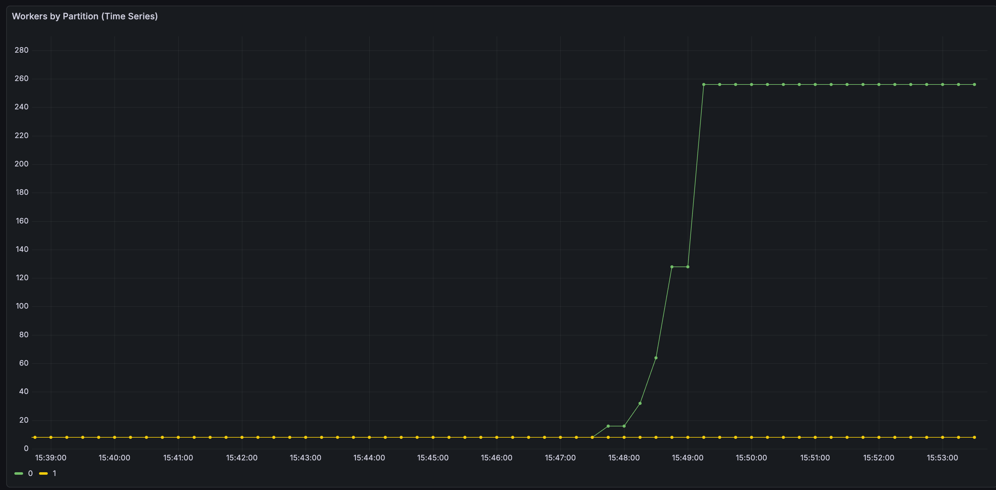
Per-partition worker counts independently scaling with load:
- Normal: maintain base worker count
- Load increase: automatic scale-up up to 8x
- Load decrease: automatic scale-down
Operational Perspective
The four-phase transition described in the deployment strategy section was completed without service interruption. Additionally, while developers previously had to manually adjust worker counts under load, the dynamic scaling system now handles load response automatically without manual intervention.
Known Limitations and Future Work
There are known limitations in the current structure:
Fixed partition count: Currently, the partition count is determined at configuration time and cannot be dynamically changed during operation. Adding or removing partitions requires redeployment.
Hot partition potential: Hash-based routing generally ensures even distribution, but in extreme cases where different TaskGroups concentrate on specific partitions, those partitions may become overloaded. However, this can be addressed by creating many logical partitions and considering techniques like shuffle sharding.
Physical partitioning transition threshold: The Redis load threshold at which to transition from logical to physical partitioning hasn’t been concretely defined. For now, we plan to monitor Redis CPU utilization and transition when necessary.
Conclusion
In this post, we addressed two problems the bulk action server faced in production — manual management of worker counts and HOL blocking from a single queue. Introducing a Redis Cluster or full distributed coordination mechanisms would have been overkill for current traffic levels, so we solved the problems with application-level keyspace separation and coordinator-based scaling.
As a result, processing time for 100,000 items was reduced from 25 minutes to 4 minutes — an 84% improvement. HOL blocking was eliminated through independent processing per partition, and worker counts now automatically adjust up to 8x based on load, eliminating the need for manual developer intervention.
We hope our experience serves as a useful reference for those considering job queue scalability or large-scale traffic processing architectures.
Thank you.
References
[1] “Head-of-line blocking,” Wikipedia. [Online]. Available: https://en.wikipedia.org/wiki/Head-of-line_blocking
[2] “Aging (scheduling),” Wikipedia. [Online]. Available: https://en.wikipedia.org/wiki/Aging_(scheduling)
[3] “Partition (database),” Wikipedia. [Online]. Available: https://en.wikipedia.org/wiki/Partition_(database)
[4] M. Kleppmann, Designing Data-Intensive Applications: The Big Ideas Behind Reliable, Scalable, and Maintainable Systems. Sebastopol, CA, USA: O’Reilly Media, 2017, ch. 6.
[5] “Sorted sets,” Redis Documentation. [Online]. Available: https://redis.io/docs/latest/develop/data-types/sorted-sets/
[6] “KRaft: Apache Kafka Without ZooKeeper,” Confluent Developer. [Online]. Available: https://developer.confluent.io/learn/kraft/
[7] “Handling billions of invocations — best practices from AWS Lambda,” AWS Compute Blog. [Online]. Available: https://aws.amazon.com/ko/blogs/compute/handling-billions-of-invocations-best-practices-from-aws-lambda/
[8] C. MacCárthaigh, “Workload isolation using shuffle-sharding,” Amazon Builders’ Library. [Online]. Available: https://aws.amazon.com/builders-library/workload-isolation-using-shuffle-sharding